Published on 25 Apr 2021 in
Machine Learning

How to do node classification and choose important features
import networkx as nx
import numpy as np
import pandas as pd
import os

import stellargraph as sg
from stellargraph.mapper import GraphSAGENodeGenerator
from stellargraph.layer import GraphSAGE

from tensorflow.keras import layers, optimizers, losses, metrics, Model
from sklearn import model_selection
from sklearn.utils import class_weight
big_df = pd.read_csv("/data/big_df_2.csv")
big_df.drop(['Unnamed: 0'], axis=1, inplace=True)
big_df['Count'] = np.abs(big_df['count']-big_df['count'].mean())/big_df['count'].std()
big_df.head()
big_df_ = big_df[big_df['depart'] == 1]
ddf = pd.read_csv("data/ddf_2.csv")
ddf.drop(['Unnamed: 0'], axis=1, inplace=True)
ddf.head()
big_G = nx.Graph()
for i in ddf.index:
    big_G.add_edge(ddf.iloc[i]['IndividualId'], ddf.iloc[i]['FatherIndividualId'])
list_nodes = list(big_df['node'])
big_G = big_G.subgraph(list_nodes)
list_nodes = list(big_G.nodes())
big_df = big_df[big_df['node'].isin(list_nodes)]
big_df = big_df.set_index('node')
train_data, test_data = model_selection.train_test_split(big_df, train_size=0.8, test_size=None, stratify=big_df['conflict'])
train_data.head()
feature_names = ['eigen', 'Count']
node_features = big_df[feature_names]
node_features.head()
node_features.describe()
node_features.info()
<class 'pandas.core.frame.DataFrame'>
Int64Index: 6780 entries, 10004 to 9972
Data columns (total 2 columns):
eigen    6780 non-null float64
Count    6780 non-null float64
dtypes: float64(2)
memory usage: 158.9 KB
G = sg.StellarGraph(big_G, node_features=node_features)
print(G.info())
StellarGraph: Undirected multigraph
 Nodes: 6780, Edges: 7623

 Node types:
  default: [6780]
    Edge types: default-default->default

 Edge types:
    default-default->default: [7623]
import matplotlib.pyplot as plt
%matplotlib inline
options = {
'node_color': 'blue',
'node_size': 100,
'width': 1,
}
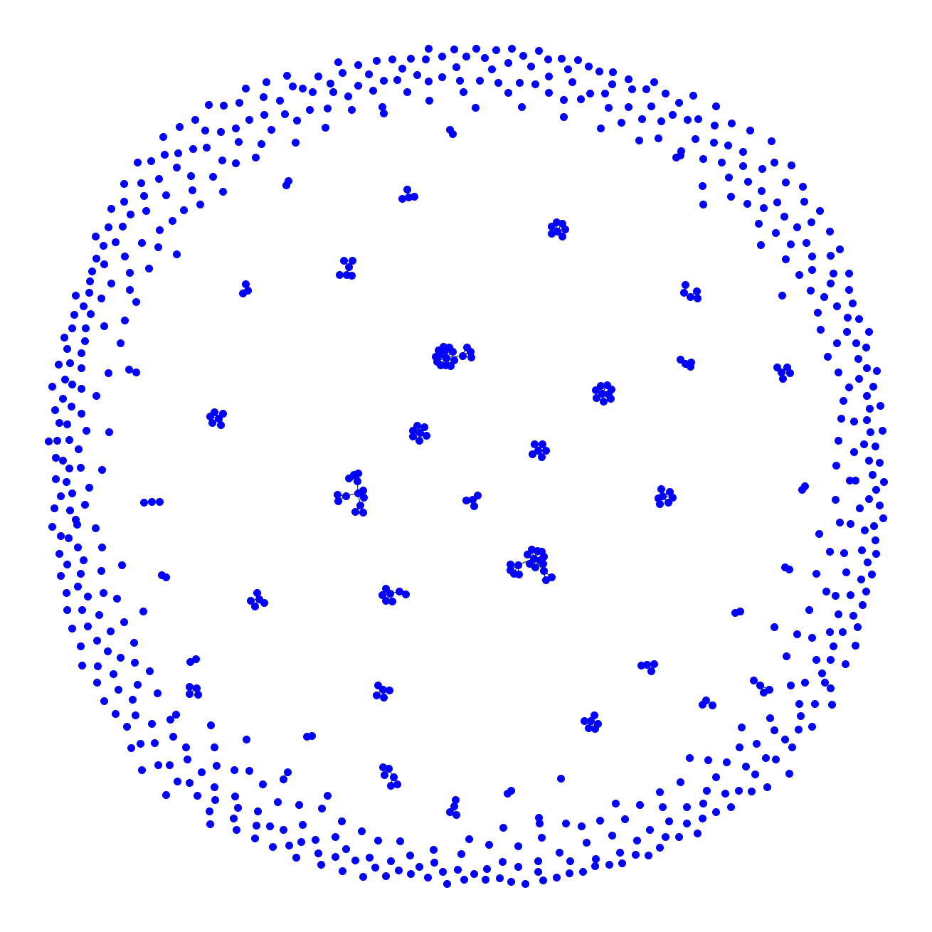
plt.figure(figsize = (18,18))
nx.draw(big_G, with_labels = False, **options)
plt.show()
from collections import Counter
Counter(train_data['conflict'])
Counter({0.0: 3250, 1.0: 2174})
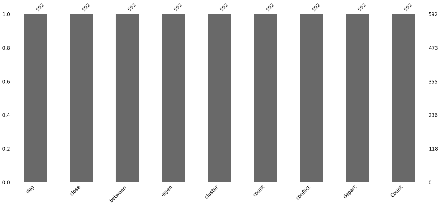
import missingno as msno
msno.bar(train_data)
print(nx.info(big_G))
Name:
Type: Graph
Number of nodes: 741
Number of edges: 164
Average degree:   0.4426
batch_size = 80; num_samples = [20, 15]
generator = GraphSAGENodeGenerator(G, batch_size, num_samples)
train_gen = generator.flow(train_data.index, np.array(train_data[["conflict"]]))
graphsage_model = GraphSAGE(
    layer_sizes=[32, 32],
    generator=train_gen,
    bias=True,
    dropout=0.1,
    #aggregator=sg.layer.graphsage.MeanAggregator
)
from tensorflow import keras
#from keras import layers, optimizers, losses, metrics, Model
x_inp, x_out = graphsage_model.build()

prediction = keras.layers.Dense(units=np.array(train_data[["conflict"]]).shape[1], activation="sigmoid")(x_out)
model = keras.Model(inputs=x_inp, outputs=prediction)

model.compile(
    optimizer=keras.optimizers.Adam(lr=0.1),
    loss=keras.losses.binary_crossentropy,
    metrics=["acc"]
)
test_gen = generator.flow(test_data.index, np.array(test_data[["conflict"]]))
history = model.fit_generator(
    train_gen,
    steps_per_epoch=len(big_df) // batch_size,
    epochs=25,
    validation_data=test_gen,
    verbose=2,
    shuffle=False
)
Epoch 1/25
84/84 - 5s - loss: 0.6341 - acc: 0.6411 - val_loss: 0.5891 - val_acc: 0.7139
Epoch 2/25
84/84 - 4s - loss: 0.5809 - acc: 0.7139 - val_loss: 0.6199 - val_acc: 0.6822
Epoch 3/25
84/84 - 4s - loss: 0.5795 - acc: 0.7123 - val_loss: 0.5800 - val_acc: 0.7205
Epoch 4/25
84/84 - 4s - loss: 0.5816 - acc: 0.7096 - val_loss: 0.5739 - val_acc: 0.7227
Epoch 5/25
84/84 - 4s - loss: 0.5811 - acc: 0.7114 - val_loss: 0.6003 - val_acc: 0.7198
Epoch 6/25
84/84 - 4s - loss: 0.5774 - acc: 0.7143 - val_loss: 0.5906 - val_acc: 0.7153
Epoch 7/25
84/84 - 4s - loss: 0.5764 - acc: 0.7176 - val_loss: 0.6150 - val_acc: 0.6807
Epoch 8/25
84/84 - 4s - loss: 0.5806 - acc: 0.7088 - val_loss: 0.5750 - val_acc: 0.7308
Epoch 9/25
84/84 - 4s - loss: 0.5741 - acc: 0.7146 - val_loss: 0.5868 - val_acc: 0.7227
Epoch 10/25
84/84 - 4s - loss: 0.5766 - acc: 0.7145 - val_loss: 0.5747 - val_acc: 0.7301
Epoch 11/25
84/84 - 4s - loss: 0.5767 - acc: 0.7117 - val_loss: 0.6028 - val_acc: 0.7050
Epoch 12/25
84/84 - 4s - loss: 0.5804 - acc: 0.7103 - val_loss: 0.5772 - val_acc: 0.7235
Epoch 13/25
84/84 - 5s - loss: 0.5744 - acc: 0.7158 - val_loss: 0.5764 - val_acc: 0.7301
Epoch 14/25
84/84 - 4s - loss: 0.5754 - acc: 0.7179 - val_loss: 0.5916 - val_acc: 0.7102
Epoch 15/25
84/84 - 4s - loss: 0.5752 - acc: 0.7155 - val_loss: 0.5748 - val_acc: 0.7271
Epoch 16/25
84/84 - 4s - loss: 0.5754 - acc: 0.7120 - val_loss: 0.5840 - val_acc: 0.7035
Epoch 17/25
84/84 - 4s - loss: 0.5795 - acc: 0.7099 - val_loss: 0.5743 - val_acc: 0.7316
Epoch 18/25
84/84 - 5s - loss: 0.5737 - acc: 0.7157 - val_loss: 0.5774 - val_acc: 0.7308
Epoch 19/25
84/84 - 5s - loss: 0.5737 - acc: 0.7158 - val_loss: 0.5821 - val_acc: 0.7257
Epoch 20/25
84/84 - 5s - loss: 0.5713 - acc: 0.7160 - val_loss: 0.5878 - val_acc: 0.7183
Epoch 21/25
84/84 - 4s - loss: 0.5744 - acc: 0.7136 - val_loss: 0.5817 - val_acc: 0.7249
Epoch 22/25
84/84 - 4s - loss: 0.5673 - acc: 0.7176 - val_loss: 0.6048 - val_acc: 0.7183
Epoch 23/25
84/84 - 4s - loss: 0.5735 - acc: 0.7187 - val_loss: 0.5852 - val_acc: 0.7286
Epoch 24/25
84/84 - 5s - loss: 0.5713 - acc: 0.7182 - val_loss: 0.6155 - val_acc: 0.6822
Epoch 25/25
84/84 - 5s - loss: 0.5758 - acc: 0.7094 - val_loss: 0.5701 - val_acc: 0.7345
import matplotlib.pyplot as plt
%matplotlib inline
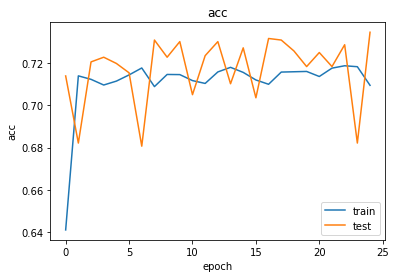
def plot_history(history):
metrics = sorted(history.history.keys())
metrics = metrics[:len(metrics)//2]
for m in metrics:
# summarize history for metric m
plt.plot(history.history[m])
plt.plot(history.history['val_' + m])
plt.title(m)
plt.ylabel(m)
plt.xlabel('epoch')
plt.legend(['train', 'test'], loc='best')
plt.show()
plot_history(history)
import multiprocessing
num_workers = multiprocessing.cpu_count()//2
train_metrics = model.evaluate_generator(train_gen, use_multiprocessing=True, workers=num_workers, verbose=1)
test_metrics = model.evaluate_generator(test_gen, use_multiprocessing=True, workers=num_workers, verbose=1)

print("\nTrain Set Metrics of the trained model:")
for name, val in zip(model.metrics_names, train_metrics):
    print("\t{}: {:0.4f}".format(name, val))

print("\nTest Set Metrics of the trained model:")
for name, val in zip(model.metrics_names, test_metrics):
    print("\t{}: {:0.4f}".format(name, val))
68/68 [==============================] - 1s 17ms/step - loss: 0.5598 - acc: 0.7303
17/17 [==============================] - 0s 22ms/step - loss: 0.5717 - acc: 0.7308

Train Set Metrics of the trained model:
	loss: 0.5598
	acc: 0.7303

Test Set Metrics of the trained model:
	loss: 0.5717
	acc: 0.7308
y_true = np.array(test_data[["conflict"]])
y_pred = model.predict_generator(test_gen)
from sklearn.metrics import classification_report
print(classification_report(np.around(y_pred), y_true))
              precision    recall  f1-score   support

         0.0       0.84      0.74      0.79       920
         1.0       0.57      0.71      0.63       436

    accuracy                           0.73      1356
   macro avg       0.70      0.73      0.71      1356
weighted avg       0.75      0.73      0.74      1356
test_metrics = model.evaluate_generator(test_gen)
print("\nTest Set Metrics:")
for name, val in zip(model.metrics_names, test_metrics):
    print("\t{}: {:0.4f}".format(name, val))
Test Set Metrics:
	loss: 0.6371
	acc: 0.5906
from sklearn.metrics import precision_recall_fscore_support
precision_recall_fscore_support(np.array(test_data['depart']), np.around(model.predict_generator(generator.flow(test_data[feature_names].index))), average='macro')
(0.8549472020841564, 0.6859450510112762, 0.7364412336901534, None)
precision_recall_fscore_support(np.array(test_data['depart']), np.around(model.predict_generator(generator.flow(test_data[feature_names].index))), average='micro')
(0.9210914454277286, 0.9210914454277286, 0.9210914454277286, None)
precision_recall_fscore_support(np.array(test_data['depart']), np.around(model.predict_generator(generator.flow(test_data[feature_names].index))), average='weighted')
(0.9126711939188366, 0.9210914454277286, 0.909333076064201, None)
num_tests = 1 # the number of times to generate predictions
all_test_predictions = [model.predict_generator(test_gen, verbose=True) for _ in np.arange(num_tests)]
17/17 [==============================] - 1s 51ms/step
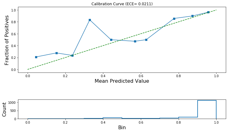
from sklearn.calibration import calibration_curve
calibration_data = [calibration_curve(y_prob=test_predictions,
                                      y_true=np.array(test_data['depart']),
                                      n_bins=10,
                                      normalize=True) for test_predictions in all_test_predictions]
from stellargraph import expected_calibration_error, plot_reliability_diagram
for fraction_of_positives, mean_predicted_value in calibration_data:
    ece_pre_calibration = expected_calibration_error(prediction_probabilities=all_test_predictions[0],
                                                     accuracy=fraction_of_positives,
                                                     confidence=mean_predicted_value)
    print('ECE: (before calibration) {:.4f}'.format(ece_pre_calibration))
ECE: (before calibration) 0.0211
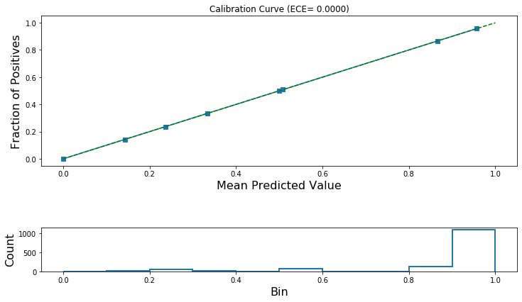
plot_reliability_diagram(calibration_data,
                         np.array(all_test_predictions[0]),
                         ece=[ece_pre_calibration])
use_platt = False  # True for Platt scaling or False for Isotonic Regression
num_tests = 1
score_model = Model(inputs=x_inp, outputs=prediction)
if use_platt:
    all_test_score_predictions = [score_model.predict_generator(test_gen, verbose=True) for _ in np.arange(num_tests)]
    all_test_probabilistic_predictions = [model.predict_generator(test_gen, verbose=True) for _ in np.arange(num_tests)]
else:
    all_test_probabilistic_predictions = [model.predict_generator(test_gen, verbose=True) for _ in np.arange(num_tests)]
17/17 [==============================] - 1s 57ms/step
# These are the uncalibrated prediction probabilities.
if use_platt:
    test_predictions = np.mean(np.array(all_test_score_predictions), axis=0)
    test_predictions.shape
else:
    test_predictions = np.mean(np.array(all_test_probabilistic_predictions), axis=0)
    test_predictions.shape
from stellargraph import IsotonicCalibration, TemperatureCalibration
if use_platt:
    # for binary classification this class performs Platt Scaling
    lr = TemperatureCalibration()
else:
    lr = IsotonicCalibration()
lr.fit(test_predictions, np.array(test_data['depart']))
lr_test_predictions = lr.predict(test_predictions)
calibration_data = [calibration_curve(y_prob=lr_test_predictions,
                                      y_true=np.array(test_data['depart']),
                                      n_bins=10,
                                      normalize=True)]
for fraction_of_positives, mean_predicted_value in calibration_data:
    ece_post_calibration = expected_calibration_error(prediction_probabilities=lr_test_predictions,
                                                      accuracy=fraction_of_positives,
                                                      confidence=mean_predicted_value)
    print('ECE (after calibration): {:.4f}'.format(ece_post_calibration))
ECE (after calibration): 0.0000
plot_reliability_diagram(calibration_data,
                         lr_test_predictions,
                         ece=[ece_post_calibration])
from sklearn.metrics import accuracy_score
y_pred = np.zeros(len(test_predictions))
if use_platt:
    # the true predictions are the probabilistic outputs
    test_predictions = np.mean(np.array(all_test_probabilistic_predictions), axis=0)
y_pred[test_predictions.reshape(-1)>0.5] = 1
print('Accuracy of model before calibration: {:.2f}'.format(accuracy_score(y_pred=y_pred,
                                                                           y_true=np.array(test_data['depart']))))
Accuracy of model before calibration: 0.92
y_pred = np.zeros(len(lr_test_predictions))
y_pred[lr_test_predictions[:,0]>0.5] = 1
print('Accuracy for model after calibration: {:.2f}'.format(accuracy_score(y_pred=y_pred, y_true=np.array(test_data['depart']))))
Accuracy for model after calibration: 0.92
Find impotant features
big_df = pd.read_csv("data/big_df_orig.csv")
big_df.drop(['Unnamed: 0'], axis=1, inplace=True)
big_df['Count'] = (big_df['Count']-big_df['Count'].mean())/big_df['Count'].std()
big_df.columns
Index(['node', 'deg', 'close', 'between', 'eigen', 'Count', 'depart'], dtype='object')
X_train, X_test, y_train, y_test = model_selection.train_test_split(big_df[['between', 'Count', 'deg', 'close', 'eigen']], big_df['depart'], test_size = 0.2)
n_train, _ = X_train.shape
print(X_train.shape, X_test.shape)
(5424, 5) (1356, 5)
n, d = big_df[['between', 'Count', 'deg', 'close', 'eigen']].shape
import matplotlib.pyplot as plt
%matplotlib inline
big_df[big_df['depart'] == 1]['between'].describe()
count    6039.000000
mean        0.001111
std         0.011457
min         0.000000
25%         0.000000
50%         0.000000
75%         0.000038
max         0.573032
Name: between, dtype: float64
big_df[big_df['depart'] == 0]['between'].describe()
count    741.000000
mean       0.000131
std        0.000813
min        0.000000
25%        0.000000
50%        0.000000
75%        0.000000
max        0.016785
Name: between, dtype: float64
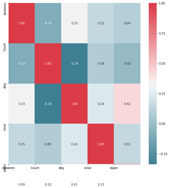
import seaborn as sns
#Create Correlation df
corr = X_train.corr()
#Plot figsize
fig, ax = plt.subplots(figsize=(10, 10))
#Generate Color Map
colormap = sns.diverging_palette(220, 10, as_cmap=True)
#Generate Heat Map, allow annotations and place floats in map
sns.heatmap(corr, cmap=colormap, annot=True, fmt=".2f")
#Apply xticks
plt.xticks(range(len(corr.columns)), corr.columns);
#Apply yticks
plt.yticks(range(len(corr.columns)), corr.columns)
#show plot
plt.show()
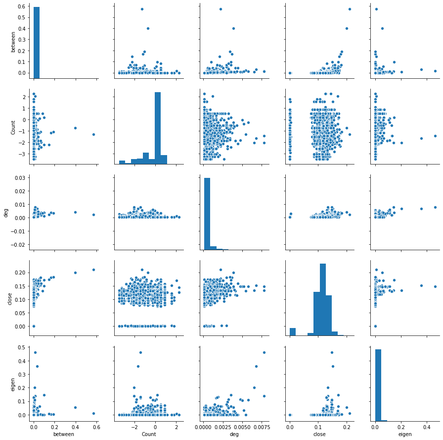
sns.pairplot(X_train)
plt.show()
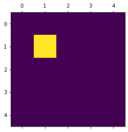
df = pd.DataFrame(X_train)
COV = df.cov()
plt.matshow(COV)
plt.show()
U, s, V = np.linalg.svd(COV, full_matrices = True)
fig = plt.figure()
plt.plot(s, 'r-o')
#plt.axvline(60, c='r')
plt.title("Valeurs singulières de la matrice de corrélation")
plt.show()
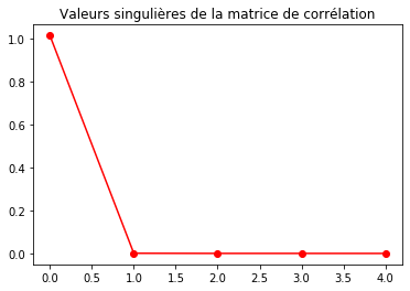
s < 0.01
array([False, True, True, True, True])
len(s)
5
s
array([1.00154518e+00, 7.86947491e-04, 1.36366655e-04, 1.23305685e-04,
       1.58050399e-07])
from sklearn.linear_model import LinearRegression, Ridge, LassoCV
regr0 = LinearRegression()
regr0.fit(X_train, y_train)

fig = plt.figure()
plt.plot(regr0.coef_, 'r-o')
plt.title("Valeurs des coefficients OLS")
plt.show()
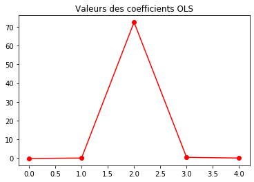
regr0.coef_
array([-2.25750655e-01,  2.61360005e-02,  7.06336051e+01,  4.24735688e-01,
       -5.19505034e-02])
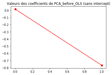
X_train_reduce = np.dot(X_train, U[:, :2])
X_test_reduce = np.dot(X_test, U[:, :2])

regr1 = LinearRegression()
regr1.fit(X_train_reduce, y_train)

fig = plt.figure()
plt.plot(regr1.coef_, 'r-o')
plt.title("Valeurs des coefficients de PCA_before_OLS (sans intercept)")
plt.show()
for y in (regr0.intercept_, regr1.intercept_, y_train.mean(axis=0)):
    print("%.3f" % y)

print("\nLes deux intercepts sont-ils égaux: %s"
      % np.isclose(regr0.intercept_, regr1.intercept_))
0.822
0.808
0.893

Les deux intercepts sont-ils égaux: False
from sklearn import preprocessing
X_train_reduce2 = preprocessing.scale(X_train_reduce)

regrtest = LinearRegression()
regrtest.fit(X_train_reduce2, y_train)

print("On vérifie l'égalité. Cette égalité est: %s."
      % np.isclose(regrtest.intercept_, np.mean(y_train)))
On vérifie l'égalité. Cette égalité est: True.
R20 = regr0.score(X_test, y_test)
R21 = regr1.score(X_test_reduce, y_test)

def MSE(y_pred, y_true):
    return np.mean((y_pred - y_true) ** 2)

pred_error0 = MSE(regr0.predict(X_test), y_test)
pred_error1 = MSE(regr1.predict(X_test_reduce), y_test)

print("Le R2 de OLS:            %.3f" % R20)
print("Le R2 de PCA before OLS: %.3f\n" % R21)
print("Le rique de prédiction de OLS calculé sur l'échantillon test:            %.2f" % pred_error0)
print("Le rique de prédiction de PCA before OLS calculé sur l'échantillon test: %.2f" % pred_error1)
Le R2 de OLS:            0.018
Le R2 de PCA before OLS: 0.008

Le rique de prédiction de OLS calculé sur l'échantillon test:            0.10
Le rique de prédiction de PCA before OLS calculé sur l'échantillon test: 0.10
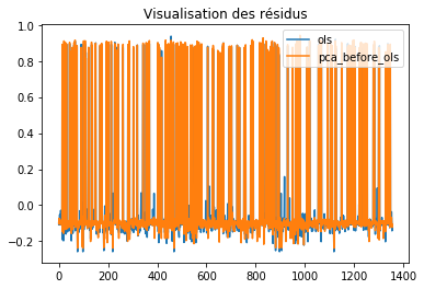
eps0 = regr0.predict(X_test) - y_test
eps1 = regr1.predict(X_test_reduce) - y_test

plt.figure()
plt.plot(eps0.values, label="ols")
plt.plot(eps1.values, label="pca_before_ols")
plt.legend(loc=1)
plt.title("Visualisation des résidus")
plt.show()
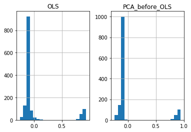
eps = pd.DataFrame(np.c_[eps0, eps1], columns=['OLS', 'PCA_before_OLS'])
eps.hist(bins=20)
plt.show()
resids = y_train

test = np.zeros((d, d))
pval_mem = np.zeros(d)
pval = np.zeros((d, d))
var_sel = []
var_remain = ['between', 'Count', 'deg', 'close', 'eigen'] #list(range(d))
in_test = []

regr = LinearRegression()
from scipy.stats import norm
d
5
for k in range(d):
    resids_mem = np.zeros((d, n_train))
    j = 0
    for i in var_remain:
        xtmp = np.array(list(X_train[i])) #X_train[:, [i]]
        xtmp = xtmp.reshape(-1, 1)
        regr.fit(xtmp, resids)

        # calcul de (x'x)
        xx = np.sum(X_train[i] ** 2) #xx = np.sum(X_train[:, i] ** 2)
        resids_mem[j, :] = regr.predict(xtmp) - resids
        sigma2_tmp = np.sum(resids_mem[j, :] ** 2) / xx
        test[k, j] = np.sqrt(n) * np.abs(regr.coef_) / (np.sqrt(sigma2_tmp))
        pval[k, j] = 2 * (1 - norm.cdf(test[k, j]))
        j = j + 1

    # separe en deux vecteurs la listes des variables séléctionnées et les autres
    best_var = np.argmax(test[k, :])
    var_sel.append(best_var)
    resids = resids_mem[best_var, :]
    pval_mem[k] = pval[k, best_var]
    var_remain = np.setdiff1d(var_remain, var_sel)

print("Voici l'ordre dans lequel les variables sont sélectionées par la méthode forward :\n\n%s" % var_sel)
Voici l'ordre dans lequel les variables sont sélectionées par la méthode forward :

[3, 3, 2, 0, 3]
fig = plt.figure()

for k in range(3):

    plt.subplot(311 + k)

    if k == 0:
        plt.title("values of the t-stat at each step")

    plt.plot(np.arange(d), test[k, :], '-o', label="step %s" % k)
    plt.plot(var_sel[k], test[k, var_sel[k]], 'r-o')
    plt.legend(loc=1)

    if k == 2:
        plt.xlabel("features")

plt.show()
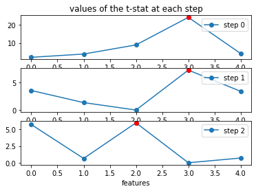
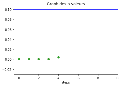
fig2 = plt.figure()

for k in range(3):
    plt.plot(np.arange(d), pval_mem, 'o')
    plt.plot([-0.5, 10], [.1, .1], color="b")
    plt.axis(xmin=-.5, xmax=10, ymin=-.03)

plt.title("Graph des p-valeurs")
plt.xlabel("steps")
plt.show()
var_sel_a = np.array(var_sel)
#print(var_sel_a,var_sel)
var_sel_def = var_sel_a[pval_mem < 0.001]

print("Il y a donc %s variables selectionnées.\nLes voici: %s" % (len(var_sel_def), var_sel_def))
There are therefore 4 selected variables.
Here they are: [3 3 2 0]
X_train.columns
Index(['between', 'Count', 'deg', 'close', 'eigen'], dtype='object')
X_train_sel = X_train[['between', 'Count']]
X_test_sel = X_test[['between', 'Count']]

regr2 = LinearRegression()
regr2.fit(X_train_sel, y_train)

print(regr2.coef_)
print(regr2.intercept_)
[0.89524856 0.0158369 ]
0.8918800888752971
pred_error_forward = MSE(regr2.predict(X_test_sel), y_test)
print("As a reminder, let us give the prediction scores obtained previouslyt.\n")

for method, error in zip(["ols           ", "pca_before_ols", "forward       "],
                         [pred_error0, pred_error1, pred_error_forward]):
    print(method + " : %.2f" % error)
As a reminder, let us give the prediction scores obtained previouslyt.

ols            : 0.10
pca_before_ols : 0.10
forward        : 0.10
np.random.seed(2)
perm = np.random.permutation(range(n_train))
q = n_train / 4.
split = np.array([0, 1, 2, 3, 4]) * q
split = split.astype(int)

for fold in range(4):
    print("The fold %s contains:\n%s\n\n" % (fold, perm[split[fold]: split[fold + 1]]))
The fold 0 contains:
[2486  738 4875 ... 3688 3723 1036]


The fold 1 containst:
[2491  857 3734 ... 4839 1668 2992]


The fold 2 contains:
[2659 1106 5196 ... 4191 3589 4707]


The fold 3 contains:
[5070 2885  249 ... 2514 3606 2575]
lasso = LassoCV()
lasso.fit(X_train, y_train)

# The estimator chose automatically its lambda:
lasso.alpha_
2.1532196265600495e-05
pred_error_lasso = MSE(lasso.predict(X_test), y_test)
print("As a reminder, let's give the scores obtained previously.\n")

for method, error in zip(["ols           ", "pca_before_ols", "forward       ",
                          "lasso         "],
                         [pred_error0, pred_error1, pred_error_forward,
                           pred_error_lasso]):
    print(method + " : %.2f" % error)
As a reminder, let's give the scores obtained previously.

ols            : 0.10
pca_before_ols : 0.10
forward        : 0.10
lasso          : 0.10
import pandas as pd
import numpy as np
from sklearn.feature_selection import SelectKBest
from sklearn.feature_selection import chi2
big_df.head()
big_df_ = big_df
big_df_[['deg', 'close', 'between', 'eigen', 'Count']] = big_df_[['deg', 'close', 'between', 'eigen', 'Count']]*1000
big_df_.head()
big_df.columns
Index(['deg', 'close', 'between', 'eigen', 'Count', 'depart'], dtype='object')
X = big_df[['deg', 'close', 'between', 'eigen', 'Count']] #independent columns
y = big_df[['depart']] #target column i.e price range
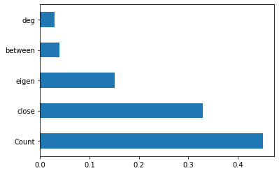
from sklearn.ensemble import ExtraTreesClassifier
import matplotlib.pyplot as plt
model = ExtraTreesClassifier()
model.fit(X,y)
print(model.feature_importances_) #use inbuilt class feature_importances of tree based classifiers
#plot graph of feature importances for better visualization
feat_importances = pd.Series(model.feature_importances_, index=X.columns)
feat_importances.nlargest(5).plot(kind='barh')
plt.show()
[0.02971642 0.32936866 0.03982511 0.1503454  0.45074441]


/home/arij/anaconda3/lib/python3.6/site-packages/sklearn/ensemble/forest.py:245: FutureWarning: The default value of n_estimators will change from 10 in version 0.20 to 100 in 0.22.
  "10 in version 0.20 to 100 in 0.22.", FutureWarning)
/home/arij/anaconda3/lib/python3.6/site-packages/ipykernel_launcher.py:6: DataConversionWarning: A column-vector y was passed when a 1d array was expected. Please change the shape of y to (n_samples,), for example using ravel().
X = big_df_[['deg', 'close', 'between', 'eigen', 'Count']]  #independent columns
y = big_df_[['depart']]    #target column i.e price range
from sklearn.ensemble import ExtraTreesClassifier
import matplotlib.pyplot as plt
model = ExtraTreesClassifier()
model.fit(X,y)
print(model.feature_importances_) #use inbuilt class feature_importances of tree based classifiers
#plot graph of feature importances for better visualization
feat_importances = pd.Series(model.feature_importances_, index=X.columns)
feat_importances.nlargest(5).plot(kind='barh')
plt.show()
[0.02684944 0.29080116 0.03635093 0.21448593 0.43151254]
import statsmodels.api as sm
from sklearn.feature_selection import RFE
from sklearn.linear_model import RidgeCV, LassoCV, Ridge, Lasso
big_df.columns
Index(['node', 'deg', 'close', 'between', 'eigen', 'Count', 'depart'], dtype='object')
#Adding constant column of ones, mandatory for sm.OLS model
X_1 = sm.add_constant(X)
#Fitting sm.OLS model
model = sm.OLS(y,X_1).fit()
model.pvalues
const      0.000000e+00
deg        1.460348e-13
close      9.604029e-04
between    5.430823e-01
eigen      7.315541e-01
Count      1.949169e-10
dtype: float64
#Backward Elimination
cols = list(X.columns)
pmax = 1
while (len(cols)>0):
    p= []
    X_1 = X[cols]
    X_1 = sm.add_constant(X_1)
    model = sm.OLS(y,X_1).fit()
    p = pd.Series(model.pvalues.values[1:],index = cols)
    pmax = max(p)
    feature_with_p_max = p.idxmax()
    if(pmax>0.05):
        cols.remove(feature_with_p_max)
    else:
        break
selected_features_BE = cols
print(selected_features_BE)
['deg', 'close', 'Count']
model = LinearRegression()
#Initializing RFE model
rfe = RFE(model, 7)
#Transforming data using RFE
X_rfe = rfe.fit_transform(X,y)
#Fitting the data to model
model.fit(X_rfe,y)
print(rfe.support_)
print(rfe.ranking_)
[ True  True  True  True  True]
[1 1 1 1 1]
#no of features
nof_list=np.arange(1,13)
high_score=0
#Variable to store the optimum features
nof=0
score_list =[]
for n in range(len(nof_list)):
    X_train, X_test, y_train, y_test = model_selection.train_test_split(X,y, test_size = 0.2, random_state = 0)
    model = LinearRegression()
    rfe = RFE(model,nof_list[n])
    X_train_rfe = rfe.fit_transform(X_train,y_train)
    X_test_rfe = rfe.transform(X_test)
    model.fit(X_train_rfe,y_train)
    score = model.score(X_test_rfe,y_test)
    score_list.append(score)
    if(score>high_score):
        high_score = score
        nof = nof_list[n]
print("Optimum number of features: %d" %nof)
print("Score with %d features: %f" % (nof, high_score))
Optimum number of features: 1
Score with 1 features: 0.005617
cols = list(X.columns)
model = LinearRegression()
#Initializing RFE model
rfe = RFE(model, 1)
#Transforming data using RFE
X_rfe = rfe.fit_transform(X,y)
#Fitting the data to model
model.fit(X_rfe,y)
temp = pd.Series(rfe.support_,index = cols)
selected_features_rfe = temp[temp==True].index
print(selected_features_rfe)
Index(['deg'], dtype='object')
reg = LassoCV()
reg.fit(X, y)
print("Best alpha using built-in LassoCV: %f" % reg.alpha_)
print("Best score using built-in LassoCV: %f" %reg.score(X,y))
coef = pd.Series(reg.coef_, index = X.columns)
Best alpha using built-in LassoCV: 0.000040
Best score using built-in LassoCV: 0.009326
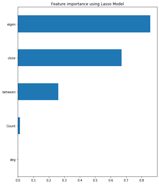
print("Lasso picked " + str(sum(coef != 0)) + " variables and eliminated the other " + str(sum(coef == 0)) + " variables")
Lasso picked 4 variables and eliminated the other 1 variables
imp_coef = coef.sort_values()
import matplotlib
matplotlib.rcParams['figure.figsize'] = (8.0, 10.0)
imp_coef.plot(kind = "barh")
plt.title("Feature importance using Lasso Model")
from feature_selector import FeatureSelector
fs = FeatureSelector(data = X, labels = y)
fs.identify_missing(missing_threshold = 0.6)
fs.missing_stats.head()
0 features with greater than 0.60 missing values.
fs.identify_collinear(correlation_threshold = 0.5)
0 features with a correlation magnitude greater than 0.50.
# Pass in the appropriate parameters
fs.identify_zero_importance(task = 'classification',
                            eval_metric = 'auc',
                            n_iterations = 10,
                             early_stopping = True)
# list of zero importance features
zero_importance_features = fs.ops['zero_importance']
Training Gradient Boosting Model

Training until validation scores don't improve for 100 rounds
Early stopping, best iteration is:
[113]	valid_0's auc: 0.918258	valid_0's binary_logloss: 0.166625
Training until validation scores don't improve for 100 rounds
Early stopping, best iteration is:
[136]	valid_0's auc: 0.920733	valid_0's binary_logloss: 0.16579
Training until validation scores don't improve for 100 rounds
Early stopping, best iteration is:
[114]	valid_0's auc: 0.933337	valid_0's binary_logloss: 0.150962
Training until validation scores don't improve for 100 rounds
Early stopping, best iteration is:
[87]	valid_0's auc: 0.92038	valid_0's binary_logloss: 0.168393
Training until validation scores don't improve for 100 rounds
Early stopping, best iteration is:
[50]	valid_0's auc: 0.92073	valid_0's binary_logloss: 0.188329
Training until validation scores don't improve for 100 rounds
Early stopping, best iteration is:
[105]	valid_0's auc: 0.913405	valid_0's binary_logloss: 0.169875
Training until validation scores don't improve for 100 rounds
Early stopping, best iteration is:
[100]	valid_0's auc: 0.944989	valid_0's binary_logloss: 0.148649
Training until validation scores don't improve for 100 rounds
Early stopping, best iteration is:
[62]	valid_0's auc: 0.903135	valid_0's binary_logloss: 0.207652
Training until validation scores don't improve for 100 rounds
Early stopping, best iteration is:
[92]	valid_0's auc: 0.938784	valid_0's binary_logloss: 0.149928
Training until validation scores don't improve for 100 rounds
Early stopping, best iteration is:
[115]	valid_0's auc: 0.910397	valid_0's binary_logloss: 0.191539

0 features with zero importance after one-hot encoding.
# plot the feature importances
fs.plot_feature_importances(threshold = 0.99, plot_n = 12)
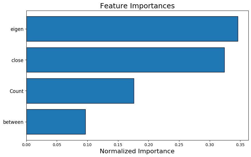
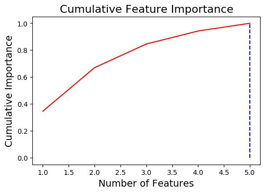
5 features required for 0.99 of cumulative importance
fs.identify_low_importance(cumulative_importance = 0.99)
4 features required for cumulative importance of 0.99 after one hot encoding.
1 features do not contribute to cumulative importance of 0.99.
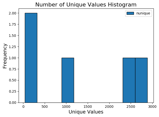
fs.identify_single_unique()
0 features with a single unique value.
fs.plot_unique()
train_removed = fs.remove(methods = 'all')
['missing', 'collinear', 'zero_importance', 'low_importance', 'single_unique'] methods have been run

Removed 1 features.
train_removed.head()
train_removed_all = fs.remove(methods = 'all', keep_one_hot=False)
['missing', 'collinear', 'zero_importance', 'low_importance', 'single_unique'] methods have been run

Removed 1 features including one-hot features.
train_removed_all.head()
fs.identify_all(selection_params = {'missing_threshold': 0.6,
                                    'correlation_threshold': 0.98,
                                    'task': 'classification',
                                    'eval_metric': 'auc',
                                    'cumulative_importance': 0.99})
0 features with greater than 0.60 missing values.

0 features with a single unique value.

0 features with a correlation magnitude greater than 0.98.

Training Gradient Boosting Model

Training until validation scores don't improve for 100 rounds
Early stopping, best iteration is:
[99]	valid_0's auc: 0.910872	valid_0's binary_logloss: 0.186959
Training until validation scores don't improve for 100 rounds
Early stopping, best iteration is:
[102]	valid_0's auc: 0.892063	valid_0's binary_logloss: 0.186904
Training until validation scores don't improve for 100 rounds
Early stopping, best iteration is:
[74]	valid_0's auc: 0.921257	valid_0's binary_logloss: 0.187569
Training until validation scores don't improve for 100 rounds
Early stopping, best iteration is:
[120]	valid_0's auc: 0.922538	valid_0's binary_logloss: 0.170568
Training until validation scores don't improve for 100 rounds
Early stopping, best iteration is:
[79]	valid_0's auc: 0.923534	valid_0's binary_logloss: 0.163693
Training until validation scores don't improve for 100 rounds
Early stopping, best iteration is:
[147]	valid_0's auc: 0.92	valid_0's binary_logloss: 0.17738
Training until validation scores don't improve for 100 rounds
Early stopping, best iteration is:
[35]	valid_0's auc: 0.916405	valid_0's binary_logloss: 0.18372
Training until validation scores don't improve for 100 rounds
Early stopping, best iteration is:
[136]	valid_0's auc: 0.910572	valid_0's binary_logloss: 0.190256
Training until validation scores don't improve for 100 rounds
Early stopping, best iteration is:
[106]	valid_0's auc: 0.919383	valid_0's binary_logloss: 0.166765
Training until validation scores don't improve for 100 rounds
Early stopping, best iteration is:
[107]	valid_0's auc: 0.914182	valid_0's binary_logloss: 0.175298

0 features with zero importance after one-hot encoding.

4 features required for cumulative importance of 0.99 after one hot encoding.
1 features do not contribute to cumulative importance of 0.99.

1 total features out of 5 identified for removal after one-hot encoding.
nodes_with_conflict = list(ddf[ddf['conflict'] == 0]['IndividualId'])
nodes_without_conflict = list(ddf[ddf['conflict'] == 1]['IndividualId'])
set(nodes_with_conflict) == set(nodes_without_conflict)
False
big_df_with_conflict = big_df[big_df['node'].isin(nodes_with_conflict)]
big_df_without_conflict = big_df[big_df['node'].isin(nodes_without_conflict)]
from pandarallel import pandarallel
pandarallel.initialize()
def inv(x):
    if x == 1:
        return 0
    elif x == 0:
        return 1
big_df['depart'] = big_df['depart'].parallel_apply(inv)
New pandarallel memory created - Size: 2000 MB
Pandarallel will run on 8 workers
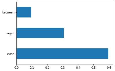
X = big_df_with_conflict[['close', 'between', 'eigen']]  #independent columns
y = big_df_with_conflict[['depart']]    #target column i.e price range
from sklearn.ensemble import ExtraTreesClassifier
import matplotlib.pyplot as plt
model = ExtraTreesClassifier()
model.fit(X,y)
print(model.feature_importances_) #use inbuilt class feature_importances of tree based classifiers
#plot graph of feature importances for better visualization
feat_importances = pd.Series(model.feature_importances_, index=X.columns)
feat_importances.nlargest(5).plot(kind='barh')
plt.show()
[0.59650393 0.09559814 0.30789793]
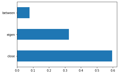
X = big_df_without_conflict[['close', 'between', 'eigen']]  #independent columns
y = big_df_without_conflict[['depart']]    #target column i.e price range
from sklearn.ensemble import ExtraTreesClassifier
import matplotlib.pyplot as plt
model = ExtraTreesClassifier()
model.fit(X,y)
print(model.feature_importances_) #use inbuilt class feature_importances of tree based classifiers
#plot graph of feature importances for better visualization
feat_importances = pd.Series(model.feature_importances_, index=X.columns)
feat_importances.nlargest(5).plot(kind='barh')
plt.show()
[0.59563847 0.07901322 0.32534832]
len(big_df_with_conflict), len(big_df_without_conflict)
(5915, 780)
fs = FeatureSelector(data = X, labels = y)
fs.identify_collinear(correlation_threshold = 0.5)
2 features with a correlation magnitude greater than 0.50.
# Pass in the appropriate parameters
fs.identify_zero_importance(task = 'classification',
                            eval_metric = 'auc',
                            n_iterations = 10,
                             early_stopping = True)
# list of zero importance features
zero_importance_features = fs.ops['zero_importance']
Training Gradient Boosting Model

Training until validation scores don't improve for 100 rounds
Early stopping, best iteration is:
[91]	valid_0's auc: 0.990654	valid_0's binary_logloss: 0.106263
Training until validation scores don't improve for 100 rounds
Early stopping, best iteration is:
[164]	valid_0's auc: 0.973625	valid_0's binary_logloss: 0.149786
Training until validation scores don't improve for 100 rounds
Early stopping, best iteration is:
[103]	valid_0's auc: 0.939869	valid_0's binary_logloss: 0.197257
Training until validation scores don't improve for 100 rounds
Early stopping, best iteration is:
[3]	valid_0's auc: 0.972772	valid_0's binary_logloss: 0.339178
Training until validation scores don't improve for 100 rounds
Early stopping, best iteration is:
[27]	valid_0's auc: 0.974852	valid_0's binary_logloss: 0.173048
Training until validation scores don't improve for 100 rounds
Early stopping, best iteration is:
[126]	valid_0's auc: 0.942535	valid_0's binary_logloss: 0.217243
Training until validation scores don't improve for 100 rounds
Early stopping, best iteration is:
[19]	valid_0's auc: 0.886644	valid_0's binary_logloss: 0.292342
Training until validation scores don't improve for 100 rounds
Early stopping, best iteration is:
[85]	valid_0's auc: 0.924411	valid_0's binary_logloss: 0.209373
Training until validation scores don't improve for 100 rounds
Early stopping, best iteration is:
[113]	valid_0's auc: 0.956186	valid_0's binary_logloss: 0.202166
Training until validation scores don't improve for 100 rounds
Early stopping, best iteration is:
[55]	valid_0's auc: 0.94248	valid_0's binary_logloss: 0.230042

0 features with zero importance after one-hot encoding.
fs.identify_low_importance(cumulative_importance = 0.99)
4 features required for cumulative importance of 0.99 after one hot encoding.
1 features do not contribute to cumulative importance of 0.99.
#train_removed_all = fs.remove(methods = 'all', keep_one_hot=False)
train_removed_all = fs.remove(methods = 'all')
['collinear', 'zero_importance', 'low_importance'] methods have been run

Removed 3 features.